|
|
|
|
|
|
| |
Finding the proper observation (or scanning) strategy is a crucial part of QUIET and, for that matter, any CMB experiment. Our choice is guided by noting that: a spatially uniform distribution maximizes sensitivity for a given integration time; a sufficiently "cross-linked" scan provides stability against time-stream filters; a convex region is best for separating E and B modes; scanning at constant elevation reduces changes in atmospheric noise; scanning as fast as possible reduces effects of 1/f noise; and a wide distribution in the angle between the detector axes and Q/U axes on the sky reduces an important systematic uncertainty. Our choice of regions will be guided by information on foreground contamination.
We use a periodical scan in azimuth (~ 1 degree/second) at high elevations (minimizing ground and atmospheric contributions), fixing the elevation and rotation angle about the optical axis.
To first detect and study the B-modes, it is necessary to make deep observations on small regions of sky. To accomplish this, we will periodically re-point and change elevation, to track regions of the sky. From experience, environmental properties are sufficiently stable on time scales up to 20 to 60 minutes, setting a natural time between re-pointings.
Parallactic Angle Coverage. QUIET radiometers measure both Q and U simultaneously. Still, in order to best separate Q and U, it is desirable to re-measure each pixel multiple times where the detector Q/U components see different combinations of the sky Q/U components, i.e. at different parallactic angles.
We have fully simulated our scan strategy and find that on average each pixel gets "hit" with parallactic angles uniformly covering a range between 70 and 170 degrees, with an average coverage of about 120 degrees. This nearly ideal situation comes without bore-sight rotations (where one fears hysteresis effects in associated offsets), something that cannot be said for polar locations.
|
| |
|
|
| |
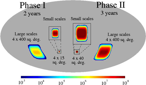
For Phase I, the 1m telescope will scan four large patches with roughly 90o difference in RA, covering a total of about 1600 square degrees. This scan is performed using the azimuthal scan described above, with an azimuthal amplitude of 10o, and re-pointing when the sky has drifted 20o. Similarly, four smaller patches within the larger patches are chosen for observations by the small-scale telescope. The scanning strategy is again identical to that described above, but by decreasing the azimuthal amplitude and the time between re-pointings, the area of each patch is decreased. By observing the same regions in both the large- and small-scale experiments, with both the Q- and W-band detectors, we are able to measure both the frequency and angular power spectra. This information will then allow us to identify a number of optimal patches for the deeper observations to take place in Phase II where the 3 2m telescopes will be scanning the same regions as in Phase I (with a factor of 20 greater depth) and the 7m telescope will be scanning 4 patches each 40 square degrees.
Distributions in the number of times we strike each pixel for each Phase of QUIET are shown in Figure 1. A simulated field including white noise based on the hit counts is shown in Figure 2.
|
| |
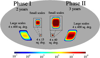 Figure 1: Number of samples (at 100 Hz) for the two phases of the observations. In each case, just one of the 4 observed patches is depicted. The patch sizes are shown to scale; the small scale regions are enlarged for added detail. For the large(small) scale, the pixel size is 14(3.5) arc minutes.
|
| |
|
|
| |
We plan to collect the data using a RAID array at the site with weekly shipments of the data to the States. It will be stored at one of our institutions (Chicago), immediately reduced and sent to the other institutions. In Phase I we expect to take about 4 TByte/year, rising to as much as 40 TByte/year in Phase II.
|
| |
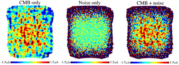
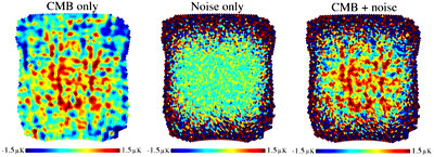 Figure 2: Simulated field (Stokes' Q) for the large-scale experiment, Phase II. The patch size is 400 square degrees. The figure illustrates the superb signal-to-noise that QUIET will obtain in the spatial domain.
|
| |
|
|
| |
Data handling and processing for QUIET will be a serious challenge. The final time stream for the polarization analysis amounts, even with moderate assumptions about the duty cycle (300 days/year, 12 hours/day), a sampling rate of 100 Hz, 2 bytes per sample, and two polarization outputs per detector (Q/U), to a rate of 1.6 GB/day (470 GB/year) for the 91-element experiment and 17 GB/day (4TB/year) for the 1000-element experiment. This puts QUIET in the same league as Planck, far beyond any previous ground- or space- based CMB experiment. Further, QUIET's exquisitely low white noise level demands similarly exquisite control of systematics.
The QUIET experiment will probe scales between l = 50 and 2500, using two different telescope designs, one for large scales and one for small scales. This difference will also reflect itself in the data analysis pipeline: two separate versions will be implemented. Specifically, the large-scale experiment will be analyzed using full-sky methods (i.e., spherical geometry, HEALPix pixelization), while the small-scale experiment will be analyzed using a flat-sky approximation. However, the algorithms will be the same for both cases, and only the implementational details will differ.
We plan two analysis centers in QUIET (Chicago and JPL) which take advantage of existing infrastructure and expertise. Several experiments have, even at current sensitivity levels, shown the benefits of parallel analyses in uncovering and quantifying systematic effects. For modest costs, we are convinced that the payoff will be significant.
|
| |
|
|
| |
To forecast QUIET's power spectrum sensitivity, we have performed simulations of the observing strategy described in the previous section. In each repointing period, we remove any ground synchronous mode from the time stream; experience from CAPMAP has shown that this is necessary to "clean" the time stream of possible ground pickup. We also remove a best-fit quadratic polynomial independently in each scan period; experience from CAPMAP has also shown that this provides sufficient high-pass filtering that the residual Time Ordered Data (TOD) noise may be treated as white. Mode removal is performed independently for each QUIET horn.
For this observing strategy and mode removal scheme, we forecast errors by constructing the dense pixel-pixel noise covariance matrix and then computing the associated band-power Fisher matrix. The expected power spectra sensitivities are shown in Figure 3 and Figure 4.
|
| |
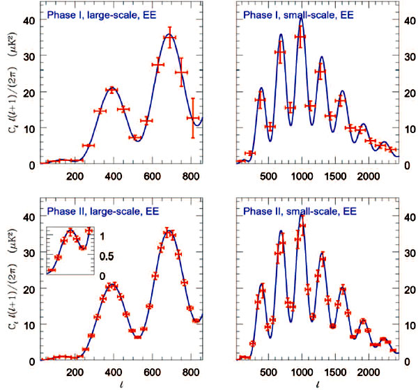
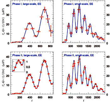 Figure 3: Results of the simulations for the EE power spectrum, Phase I and II, large and small scale telescopes. The simulations are for the observing strategy described in the previous section, including offset removals for each detector and marginalization over power in adjacent bands (the band-power correlations are less than 10%). For Phase II, large scale, a detail of the expected errors for the first peak is shown.
|
| |
We emphasize that these forecasts incorporate several effects which might not be accounted for in a simpler treatment. Since exact pixel-pixel covariance matrices in the QUIET survey region are used, the effect of "E-B leakage", or downgraded B-mode sensitivity due to boundary conditions, has been incorporated into the forecasts. Additionally, the loss of sensitivity caused by mode removal in the time domain, as described in the previous paragraph, is reflected in the noise covariance matrix used to compute the error bars. Finally, when showing an error bar for each band-power, we have marginalized over power in adjacent bands, and in the case of B modes, marginalized over E power as well. We will be discussing the effects of foregrounds later in this proposal.
From Figure 3, it is clear that we will measure the EE power spectrum very accurately from l=50 to above 2500, by combining results from the 2- and 7-meter telescope data. This lever arm coupled with the accuracy of the measurements will yield a very precise determination of the tilt to the spectrum, to constrain inflationary models. From inspecting the noise levels, it is clear that we go far deeper than Planck in both our fields. This means we will have an extended reach for new physical effects, be it unexpected features of the power-spectrum, non-Gaussian effects in the fluctuations, or simply new sources of foregrounds, effects that experiments with lower sensitivity would not be able to detect.
|
| |
Lensing Power. The plots on the right hand side of Figure 4 show our expected sensitivity to the lensing power, in both Phase I and II. The curves show our expected measurements of the power at each multipole, including the relatively large contribution from sample variance. We have distinguished between "lensing power", the expected constraint on the amplitude of the BB power spectrum, and "lensing significance", the expected significance of detecting a nonzero B-mode component in the CMB (assuming that lensing is the only source of B modes). A non-zero neutrino mass affects the growth of structure and the effects on the lensing power have been documented in the literature. In estimates of our sensitivity to the (mean) neutrino mass, we have included the effects of the expected correlations among the (non-Gaussian) power spectra in the several l-bins.
|
| |
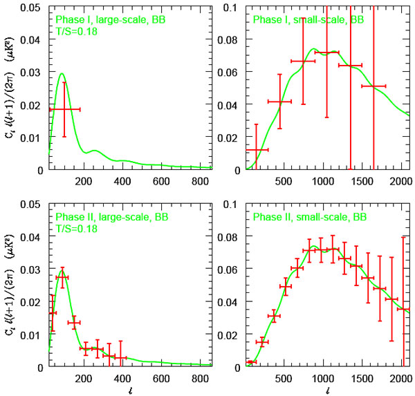
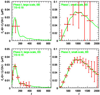 Figure 4: Results as in Figure 3 for the BB power spectra. On the right the smooth curve is the expected spectrum from lensing; on the left only the expected spectrum from gravitational waves corresponding to T/S=0.18 is shown. At this value, we have a 5σ detection in Phase I as described in the text. The simulations are for the observing strategy described in the previous section, including such often-neglected effects as: offset removals for each detector (the source of the increase in error for the lowest l bin, lower-left plot); the effects of "E-B leakage"; and marginalization over power in adjacent (E and B) bands (the band-power correlations are again less than 10%.).
|
| |
Gravity Waves. For both phases of QUIET, we have used simulations to compute the minimum T/S for which the gravity wave component of the B modes is detectable at a level of 5σ. In phase II, achieving the forecasted sensitivity of T/S = 0.009 will require overcoming several data analysis challenges. First, the quoted sensitivity neglects residual contamination of the gravity wave B mode signal by lensing B modes. Naive signal-to-noise considerations, treating the lensing B modes as an extra source of Gaussian noise, show that the resulting loss of sensitivity to T/S is 20% for T/S = 0.009. This can potentially be improved by using "cleaning" algorithms to separate the gravity wave and lensing B modes, but we have not yet performed a detailed investigation. First, it has recently been argued that pseudo-Cl estimators, as currently formulated in the literature, cannot achieve sensitivity better than T/S = 0.05, because these estimators do not achieve optimal separation of E and B. (The Fisher matrix calculations implicitly assume optimal quadratic estimators, and therefore do not suffer from this limit.) Therefore, some modification of the pseudo-Cl framework will presumably be needed to achieve the exquisite sensitivity to T/S made possible by the QUIET instrument.
We have also used simulations to forecast error bars on the gravity wave B mode power spectrum. The results are shown on the left side of Figure 4; in the simulations, we have used T/S = 0.18, a value allowed by all previous measurements, in computing the expected B mode power spectrum. For this value of T/S, we can detect gravity waves in just Phase I at the 5σ level.
For now we can say that for Phase I our sensitivities are at least as good as the best of our competition- QUaD and BICEP; for Phase II they are about 20 times better. And, while Planck has good sensitivity to T/S, it comes almost exclusively from the re-ionization bump whereas our sensitivity comes from the surface of last scattering. Seeing both signatures is required for a convincing signature of this important phenomenon.
|
| |
|
|
|